

Table of Contents
Discounted Cash Flow Formula: Definition, Calculation and Example
- 5 min read
- Authored & Reviewed by: CLFI Team
The Discounted Cash Flow (DCF) method lies at the heart of modern valuation. It provides a structured way to determine what a business, project, or investment is worth today by forecasting its future cash flows and adjusting them to present value. Rather than focusing on accounting profits, DCF captures how much cash a business will generate — and how the time value of money affects that stream.
Understanding how to calculate DCF is essential for corporate finance professionals, investors, and executives making strategic decisions on capital investment or acquisitions. The method underpins valuations used in mergers and acquisitions, private equity, and financial modelling — and connects directly with key concepts such as WACC, IRR, and Free Cash Flow (FCF).
In this article, we break down the DCF formula, explain its components, and show how to calculate it step by step — supported by a numerical example and a short interpretation to help you read results in practice.
The foundations of discounted cash flow analysis, including the treatment of cash flows and discounting, are developed within the Business Valuation Executive Course.
Table of Contents
What Is Discounted Cash Flow (DCF)?
Discounted Cash Flow, or DCF, is a valuation method used to estimate the intrinsic value of an investment based on its expected future cash flows. The central idea is that the value of money changes over time — a pound received today is worth more than the same pound received in five years. This principle, known as the time value of money, underpins all corporate finance valuation models.
Definition:
Discounted Cash Flow (DCF)
A valuation technique that determines the present value of expected future cash flows using a discount rate that reflects the investment’s risk and the time value of money.
DCF allows investors and decision-makers to assess whether an investment is worth pursuing by comparing its intrinsic value to its market price. If the DCF value exceeds the market value, the investment may be undervalued, suggesting potential upside. Conversely, if the DCF value is lower, it may be overvalued, signalling risk or inflated expectations.
In corporate settings, DCF is used to value entire businesses, individual projects, or specific assets such as a factory, a brand, or a patent. It plays a central role in mergers and acquisitions, capital budgeting, and private equity analysis — where professionals seek to forecast Free Cash Flow (FCF) over time and discount those amounts at the appropriate Weighted Average Cost of Capital (WACC).
For example, when an investor considers acquiring a coffee chain, they forecast the cash the business will generate from operations each year, then discount those cash flows back to today’s value using a rate that reflects the risk of the investment and the cost of financing. The result represents the business’s intrinsic value, independent of market noise or short-term sentiment.
Programme Content Overview
The Executive Certificate in Corporate Finance, Valuation & Governance delivers a full business-school-standard curriculum through flexible, self-paced modules. It covers five integrated courses — Corporate Finance, Business Valuation, Corporate Governance, Private Equity, and Mergers & Acquisitions — each contributing a defined share of the overall learning experience, combining academic depth with practical application.

Chart: Percentage weighting of each core course within the CLFI Executive Certificate curriculum.
Price Is a Data Point. Value Is a Decision.
Learn more through the Executive Certificate in Corporate Finance, Valuation & Governance – a structured programme integrating governance, finance, valuation, and strategy.
The DCF Formula Explained
At its core, the Discounted Cash Flow model calculates today’s value of a series of future cash flows. Each future cash flow is divided by a factor that represents how much less valuable that amount is in today’s terms. The discounting factor depends on the discount rate, often represented by the company’s Weighted Average Cost of Capital (WACC).
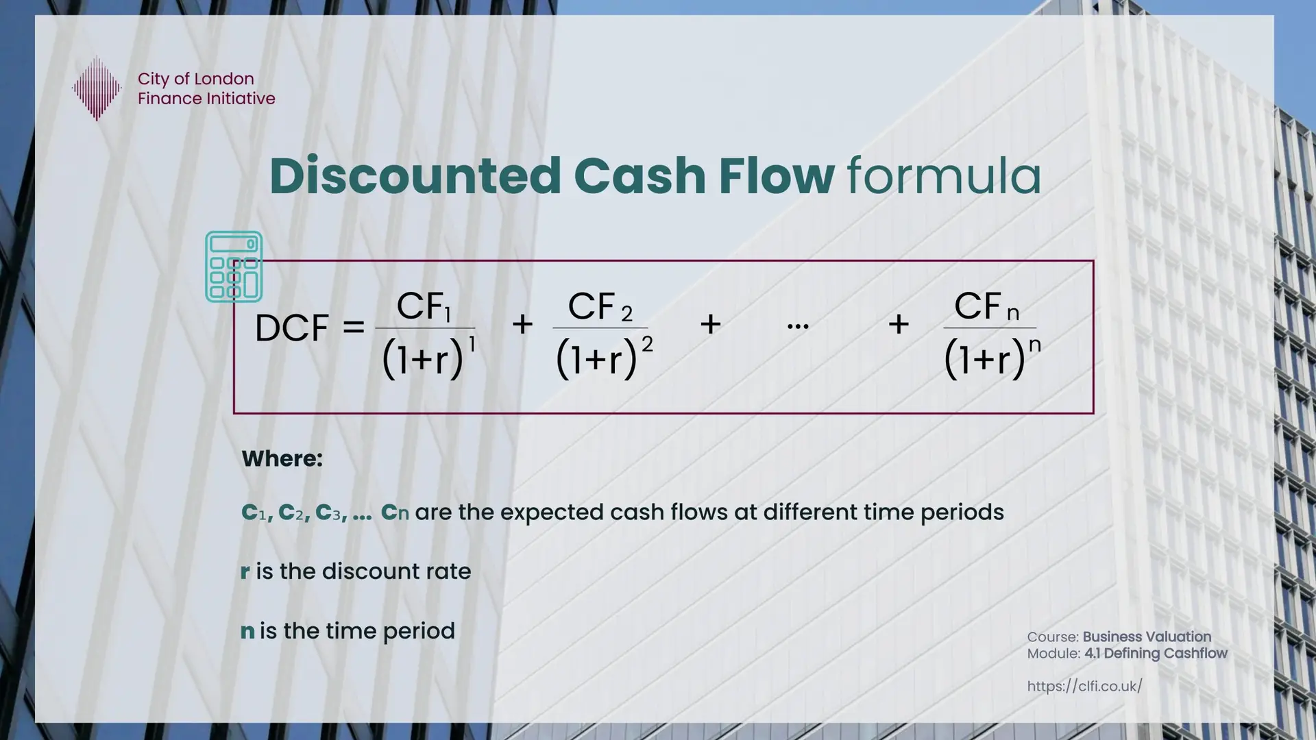
DCF Formula:
DCF = CF₁ / (1 + r)¹ + CF₂ / (1 + r)² + … + CFₙ / (1 + r)ⁿ + TV / (1 + r)ⁿ
Where:
| CF₁ … CFₙ | Projected free cash flows for each year of the forecast period |
| r | Discount rate (usually the WACC, reflecting both debt and equity costs) |
| TV | Terminal Value — the value of all cash flows beyond the forecast period |
The terminal value (TV) captures the continuing value of the business after the explicit forecast horizon, often representing the majority of total value in a DCF. It can be estimated using either a perpetuity growth model or an exit multiple approach linked to industry benchmarks such as EV/EBITDA multiples.
Because the DCF model depends on assumptions about future performance and discount rates, small changes in inputs can significantly alter the valuation outcome. This sensitivity is why financial analysts typically test several scenarios — adjusting growth rates, margins, or discount rates to observe how intrinsic value changes.
Aurra Textiles Ltd.
Calculating Return on Capital Employed (ROCE)
Compute ROCE
Final Metric Summary
Steps to Calculate DCF
Calculating a Discounted Cash Flow involves a structured, five-step process. While the underlying mathematics are straightforward, the quality of inputs — particularly the cash flow forecasts and discount rate — determines how credible the result will be. The steps below summarise the professional approach used in corporate finance and valuation practice.
Step 1: Forecast Free Cash Flows (FCF)
Start by projecting the company’s Free Cash Flow to the Firm (FCFF) — the cash available to both debt and equity holders after accounting for operating expenses, taxes, and reinvestment needs. These forecasts typically span 3 to 10 years, depending on the business’s maturity and predictability.
Formula:
FCF = EBIT × (1 − Tax Rate) + Depreciation − Capital Expenditure − ΔWorking Capital
Step 2: Estimate the Discount Rate (WACC)
Next, calculate the Weighted Average Cost of Capital (WACC). It reflects the blended cost of equity and debt financing, adjusted for the company’s risk profile and market conditions. A higher perceived risk leads to a higher discount rate, reducing the present value of cash flows.
Step 3: Discount the Cash Flows
Each forecasted cash flow is divided by (1 + WACC)t, where t represents the year number. This adjusts future values to reflect today’s equivalent, considering both risk and time. The further into the future a cash flow occurs, the smaller its present value will be.
Step 4: Calculate the Terminal Value (TV)
Once the explicit forecast period ends, a Terminal Value is calculated to capture the continuing value of the company. Two main methods exist:
- Perpetuity Growth Method: assumes the business grows at a steady rate (g) indefinitely.
TV = (FCFn × (1 + g)) / (WACC − g) - Exit Multiple Method: applies a valuation multiple, such as EV/EBITDA, based on comparable industry transactions.
Step 5: Sum the Present Values
Finally, add all the discounted cash flows and the discounted terminal value. The total equals the Enterprise Value (EV) of the firm. From there, subtract net debt to obtain the Equity Value — which can then be divided by the number of shares to estimate intrinsic value per share.
This process provides a logically consistent framework for valuation, linking operational performance (through FCF) to market expectations (through WACC and terminal value). While it involves assumptions, DCF remains one of the most transparent and academically grounded methods for estimating intrinsic value.
To anchor the method, consider a mid-market UK company with five explicit years of forecast free cash flow to the firm and a stable growth profile thereafter. We use a WACC of 10 percent and a long-term growth rate of 3 percent. All figures are in millions of pounds, rounded to one decimal place for readability.
DCF Valuation Case
Five year FCFF forecast, WACC 10 percent, terminal growth 3 percent
Present value of explicit FCFF (Years 1 to 5)
Terminal value at Year 5 and present value
Enterprise value, equity value, value per share
Final Metrics Summary
Interpretation. The valuation is driven mainly by the terminal value, which contributes about 75.5% of enterprise value. This is common in stable, cash-generative businesses and highlights how sensitive DCF outcomes are to the long term growth and the discount rate. The explicit period contributes 24.5%, which still provides a useful anchor because it reflects near term operating performance that management can influence more directly.
With net debt of £20.0m the equity value is £100.97m, which implies an intrinsic value per share of £2.02 for 50.0m shares. In practice, a professional model would test alternative scenarios for growth, margins, capital expenditure, and WACC, then observe how intrinsic value responds. The goal is not a single number, it is a range that supports decision making on investment, pricing, or deal structure.
DCF Formula vs Other Valuation Methods
The discounted cash flow formula is one of three primary valuation approaches used in corporate finance and M&A practice. Understanding where each method is strongest — and where it has limitations — helps analysts and executives apply DCF output with appropriate confidence rather than treating it as a self-contained conclusion.
Trading comparables value a business using multiples derived from listed peer companies, with EV/EBITDA being the most widely applied measure in UK mid-market and large-cap transactions. This approach is fast and market-calibrated, reflecting what buyers and sellers are currently paying in public markets, but it depends on the availability of genuinely comparable companies and moves in line with broader market sentiment regardless of whether that sentiment reflects underlying value.
Transaction comparables work on the same principle but draw from recent acquisitions of similar businesses rather than listed prices. Because they capture actual deal prices, they typically incorporate a control premium and are more directly relevant for pricing an acquisition. Their limitation is that they embed the deal conditions of the period in which the transactions occurred, including leverage availability, buyer appetite, and market timing, which may or may not reflect the environment in which a new deal is being structured.
The DCF formula stands apart from both approaches because it derives value from the business's own projected cash flows rather than from external market pricing. In practice, experienced analysts triangulate across all three methods, using the DCF as a fundamentals anchor, trading and transaction comparables as market context, and the gap between the two as a diagnostic signal about whether the market is pricing the sector above or below intrinsic value.
| Method | Value Basis | Strongest When | Key Limitation |
|---|---|---|---|
| DCF Formula | Projected free cash flows discounted to present value | Comparables are scarce or when testing whether a price is supported by fundamentals | Highly sensitive to WACC and terminal growth rate assumptions |
| Trading Comparables | Listed peer company multiples (EV/EBITDA, EV/Revenue) | A liquid peer set is available and a fast, market-calibrated benchmark is needed | Moves with market sentiment regardless of whether that sentiment reflects fundamental value |
| Transaction Comparables | Recent acquisition multiples including control premium | Pricing an acquisition and understanding what buyers have recently paid for similar assets | Embeds historical deal conditions that may not reflect current leverage availability or buyer appetite |
Advantages and Limitations of DCF
The Discounted Cash Flow approach remains the foundation of professional valuation because it connects projected financial performance directly with value creation. It forces analysts and executives to translate business narratives — such as expansion, efficiency, or innovation — into measurable financial outcomes. Yet, its strength in transparency can also expose it to subjectivity, particularly when assumptions are stretched.
Advantages
DCF is highly flexible and can be adapted to almost any type of investment, from early-stage ventures to mature infrastructure assets. It isolates intrinsic value from market sentiment, allowing decision-makers to focus on fundamentals rather than short-term volatility. By discounting future cash flows at a risk-adjusted rate, it captures the opportunity cost of capital and enables consistent comparison between projects. Moreover, the DCF framework aligns naturally with strategic planning, capital budgeting, and performance management, linking financial forecasts to value outcomes.
Limitations
Despite its conceptual rigour, DCF is sensitive to estimation errors. A small change in discount rate or terminal growth can materially shift the valuation, sometimes by double-digit percentages. This makes scenario and sensitivity analysis essential for credible results. The method also assumes that forecasts are internally consistent — that revenue growth, margins, capital expenditure, and working capital all evolve logically together. If these drivers are misaligned, the output can appear precise but be fundamentally misleading.
DCF also tends to be less reliable for businesses with unpredictable or cyclical cash flows, such as early-stage startups or commodities producers. In those cases, analysts often combine DCF with relative valuation multiples, such as EV/EBITDA or price-to-earnings, to cross-check results and ensure realism. Used with discipline, the method remains the cornerstone of valuation analysis, but it requires both financial competence and sound judgment.
In Practice: Using DCF in Strategic Decisions
In executive decision-making, DCF analysis is not only a valuation tool but a strategic framework. It enables leaders to test how operational choices — such as entering a new market, automating production, or acquiring a competitor — translate into long-term value. Each assumption about revenue, cost, or capital intensity must eventually flow into cash, making the DCF model a mirror of strategic realism.
Boards and investors often use DCF outputs to benchmark performance against required returns, determine whether projects meet investment hurdles, or guide negotiations in mergers and acquisitions. The same logic applies to capital allocation: a project delivering a positive net present value (NPV) at the firm’s WACC creates value, while one below the hurdle erodes it. Because every cash flow and discount rate reflects an underlying decision, the model helps bring quantitative discipline to qualitative judgment.
In practice, finance leaders rarely rely on a single DCF outcome. They develop scenarios — base, optimistic, and downside — to reflect uncertainty and to evaluate resilience. This approach ensures that boardroom discussions focus not only on value potential but also on risk absorption, liquidity, and long-term sustainability. Properly applied, the DCF framework converts forecasts into a transparent, strategic conversation about value creation.
Learn more in the Executive Certificate in Corporate Finance, Valuation & Governance.